Combining/merging
Because all uncertainties are handled using a resampling approach, it is trivial to combine or merge uncertain values of different types into a single uncertain value.
Nomenclature
Depending on your data, you may want to choose of one the following ways of representing multiple uncertain values as one:
- Combining. An ensemble of uncertain values is represented as a weighted population. This approach is nice if you want to impose expert-opinion on the relative sampling probabilities of uncertain values in the ensemble, but still sample from the entire supports of each of the furnishing values. This introduces no additional approximations besides what is already present at the moment you define your uncertain values.
- Merging. Multiple uncertain values are merged using a kernel density estimate to the overall distribution. This approach introduces approximations beyond what is present in the uncertain values when you define them.
Combining uncertain values: the population approach
Combining uncertain values is done by representing them as a weighted population of uncertain values, which is illustrated in the following example:
1 2 3 4 5 6 7 8 9 10 11 | # Assume we have done some analysis and have three points whose uncertainties # significantly overlap. v1 = UncertainValue(Normal(0.13, 0.52)) v2 = UncertainValue(Normal(0.27, 0.42)) v3 = UncertainValue(Normal(0.21, 0.61)) # Give each value equal sampling probabilities and represent as a population pop = UncertainValue([v1, v2, v3], [1, 1, 1]) # Let the values v1, v2 and v3 be sampled with probability ratios 1-2-3 pop = UncertainValue([v1, v2, v3], [1, 2, 3]) |

This is not restricted to normal distributions! We can combine any type of value in our population, even populations!
1 2 3 4 5 6 7 8 9 10 11 12 13 14 15 16 17 18 | # Consider a population of normal distributions, and a gamma distribution v1 = UncertainValue(Normal(0.265, 0.52)) v2 = UncertainValue(Normal(0.311, 0.15)) v3 = UncertainValue([v1, v2], [2, 1]) v4 = UncertainValue(Gamma(0.5, -1)) pts = [v1, v4] wts = [2, 1] # New population is a nested population with unequal weights pop = UncertainValue(pts, wts) d1 = density(resample(pop, 20000), label = "population") d2 = plot() density!(d2, resample(pop[1], 20000), label = "v1") density!(d2, resample(pop[2], 20000), label = "v2") plot(d1, d2, layout = (2, 1), xlabel = "Value", ylabel = "Density", link = :x, xlims = (-2.5, 2.5)) |

This makes it possible treat an ensemble of uncertain values as a single uncertain value.
With equal weights, this introduces no bias beyond what is present in the data, because resampling is done from the full supports of each of the furnishing values. Additional information on relative sampling probabilities, however, be it informed by expert opinion or quantative estimates, is easily incorporated by adjusting the sampling weights.
Merging uncertain values: the kernel density estimation (KDE) approach
Merging multiple uncertain values could be done by fitting a model distribution to the values. Using any specific theoretical distribution as a model for the combined uncertainty, however, is in general not possible, because the values may have different types of uncertainties.
Thus, in this package, kernel kernel density estimation is used to merge multiple uncertain values. This has the advantage that you only have to deal with a single estimate to the combined distribution, but introduces bias because the distribution is estimated and the shape of the distribution depends on the parameters of the KDE procedure.
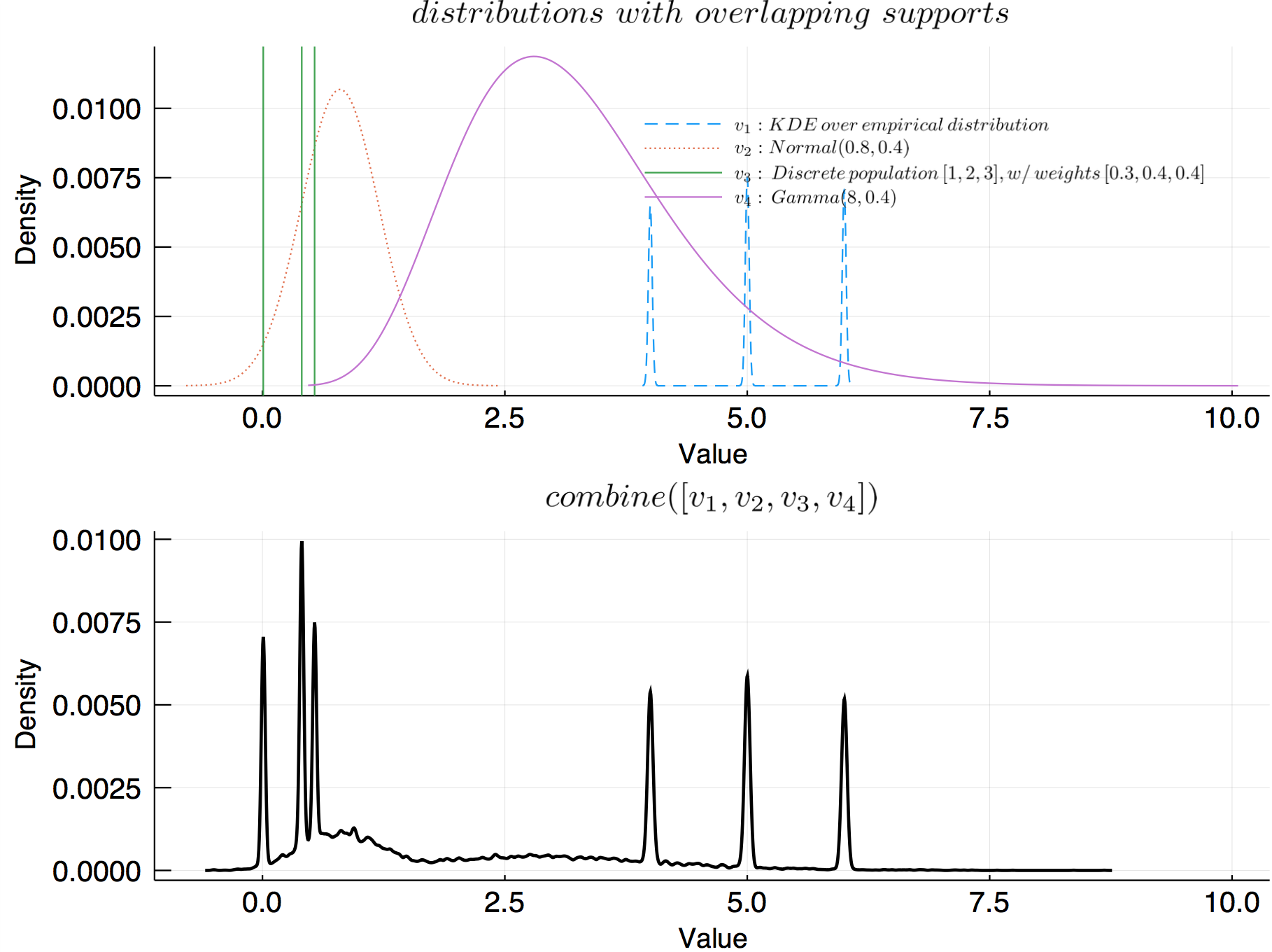
Without weights
When no weights are provided, the combined value is computed by resampling each of the N uncertain values n/N times, then combining using kernel density estimation.
#
UncertainData.combine — Method.
1 2 | combine(uvals::Vector{AbstractUncertainValue}; n = 10000*length(uvals), bw::Union{Nothing, Real} = nothing) |
Combine multiple uncertain values into a single uncertain value. This is done by resampling each uncertain value in uvals, n times each, then pooling these draws together. Finally, a kernel density estimate to the final distribution is computed over those draws.
The KDE bandwidth is controlled by bw. By default, bw = nothing; in this case, the bandwidth is determined using the KernelDensity.default_bandwidth function.
Tip
For very wide, close-to-normal distributions, the default bandwidth may work well. If you're combining very peaked distributions or discrete populations, however, you may want to lower the bandwidth significantly.
Example
1 2 3 4 5 6 7 8 | v1 = UncertainValue(Normal, 1, 0.3) v2 = UncertainValue(Normal, 0.8, 0.4) v3 = UncertainValue([rand() for i = 1:3], [0.3, 0.3, 0.4]) v4 = UncertainValue(Normal, 3.7, 0.8) uvals = [v1, v2, v3, v4]; combine(uvals) combine(uvals, n = 20000) # adjust number of total draws |
Weights dictating the relative contribution of each uncertain value into the combined value can also be provided. combine works with ProbabilityWeights, AnalyticWeights, FrequencyWeights and the generic Weights.
Below shows an example of combining
1 2 3 4 5 6 7 8 9 10 11 12 13 14 15 | v1 = UncertainValue(rand(1000)) v2 = UncertainValue(Normal, 0.8, 0.4) v3 = UncertainValue([rand() for i = 1:3], [0.3, 0.3, 0.4]) v4 = UncertainValue(Normal, 3.7, 0.8) uvals = [v1, v2, v3, v4] p = plot(title = L"distributions \,\, with \,\, overlapping \,\, supports") plot!(v1, label = L"v_1", ls = :dash) plot!(v2, label = L"v_2", ls = :dot) vline!(v3.values, label = L"v_3") # plot each possible state as vline plot!(v4, label = L"v_4") pcombined = plot(combine(uvals), title = L"merge(v_1, v_2, v_3, v_4)", lc = :black, lw = 2) plot(p, pcombined, layout = (2, 1), link = :x, ylabel = "Density") |
With weights
Weights, ProbabilityWeights and AnalyticWeights are functionally the same. Either may be used depending on whether the weights are assigned subjectively or quantitatively. With FrequencyWeights, it is possible to control the exact number of draws from each uncertain value that goes into the draw pool before performing KDE.
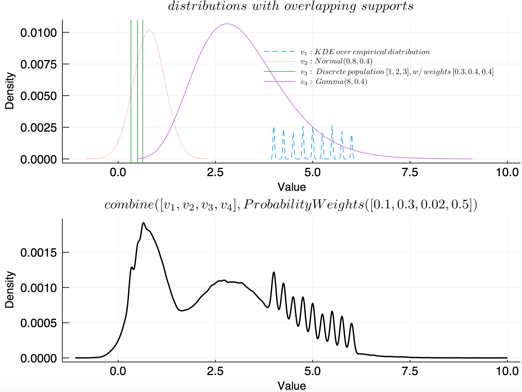
ProbabilityWeights
#
UncertainData.combine — Method.
1 2 3 | combine(uvals::Vector{AbstractUncertainValue}, weights::ProbabilityWeights; n = 10000*length(uvals), bw::Union{Nothing, Real} = nothing) |
Combine multiple uncertain values into a single uncertain value. This is done by resampling each uncertain value in uvals proportionally to the provided relative analytic weights indicating their relative importance (these are normalised by default, so don't need to sum to 1), then pooling these draws together. Finally, a kernel density estimate to the final distribution is computed over the n total draws.
Providing ProbabilityWeights leads to the exact same behaviour as for AnalyticWeights, but may be more appropriote when, for example, weights have been determined quantitatively.
The KDE bandwidth is controlled by bw. By default, bw = nothing; in this case, the bandwidth is determined using the KernelDensity.default_bandwidth function.
Tip
For very wide, close-to-normal distributions, the default bandwidth may work well. If you're combining very peaked distributions or discrete populations, however, you may want to lower the bandwidth significantly.
Example
1 2 3 4 5 6 7 8 9 | v1 = UncertainValue(Normal, 1, 0.3) v2 = UncertainValue(Normal, 0.8, 0.4) v3 = UncertainValue([rand() for i = 1:3], [0.3, 0.3, 0.4]) v4 = UncertainValue(Normal, 3.7, 0.8) uvals = [v1, v2, v3, v4]; # Two difference syntax options combine(uvals, ProbabilityWeights([0.2, 0.1, 0.3, 0.2])) combine(uvals, pweights([0.2, 0.1, 0.3, 0.2]), n = 20000) # adjust number of total draws |
For example:
1 2 3 4 5 6 7 8 9 10 11 12 13 14 15 16 17 18 19 20 21 22 23 24 | v1 = UncertainValue(UnivariateKDE, rand(4:0.25:6, 1000), bandwidth = 0.02) v2 = UncertainValue(Normal, 0.8, 0.4) v3 = UncertainValue([rand() for i = 1:3], [0.3, 0.3, 0.4]) v4 = UncertainValue(Gamma, 8, 0.4) uvals = [v1, v2, v3, v4]; p = plot(title = L"distributions \,\, with \,\, overlapping \,\, supports") plot!(v1, label = L"v_1: KDE \, over \, empirical \, distribution", ls = :dash) plot!(v2, label = L"v_2: Normal(0.8, 0.4)", ls = :dot) # plot each possible state as vline vline!(v3.values, label = L"v_3: \, Discrete \, population\, [1,2,3], w/ \, weights \, [0.3, 0.4, 0.4]") plot!(v4, label = L"v_4: \, Gamma(8, 0.4)") pcombined = plot( combine(uvals, ProbabilityWeights([0.1, 0.3, 0.02, 0.5]), n = 100000, bw = 0.05), title = L"combine([v_1, v_2, v_3, v_4], ProbabilityWeights([0.1, 0.3, 0.02, 0.5])", lc = :black, lw = 2) plot(p, pcombined, layout = (2, 1), size = (800, 600), link = :x, ylabel = "Density", tickfont = font(12), legendfont = font(8), fg_legend = :transparent, bg_legend = :transparent) |
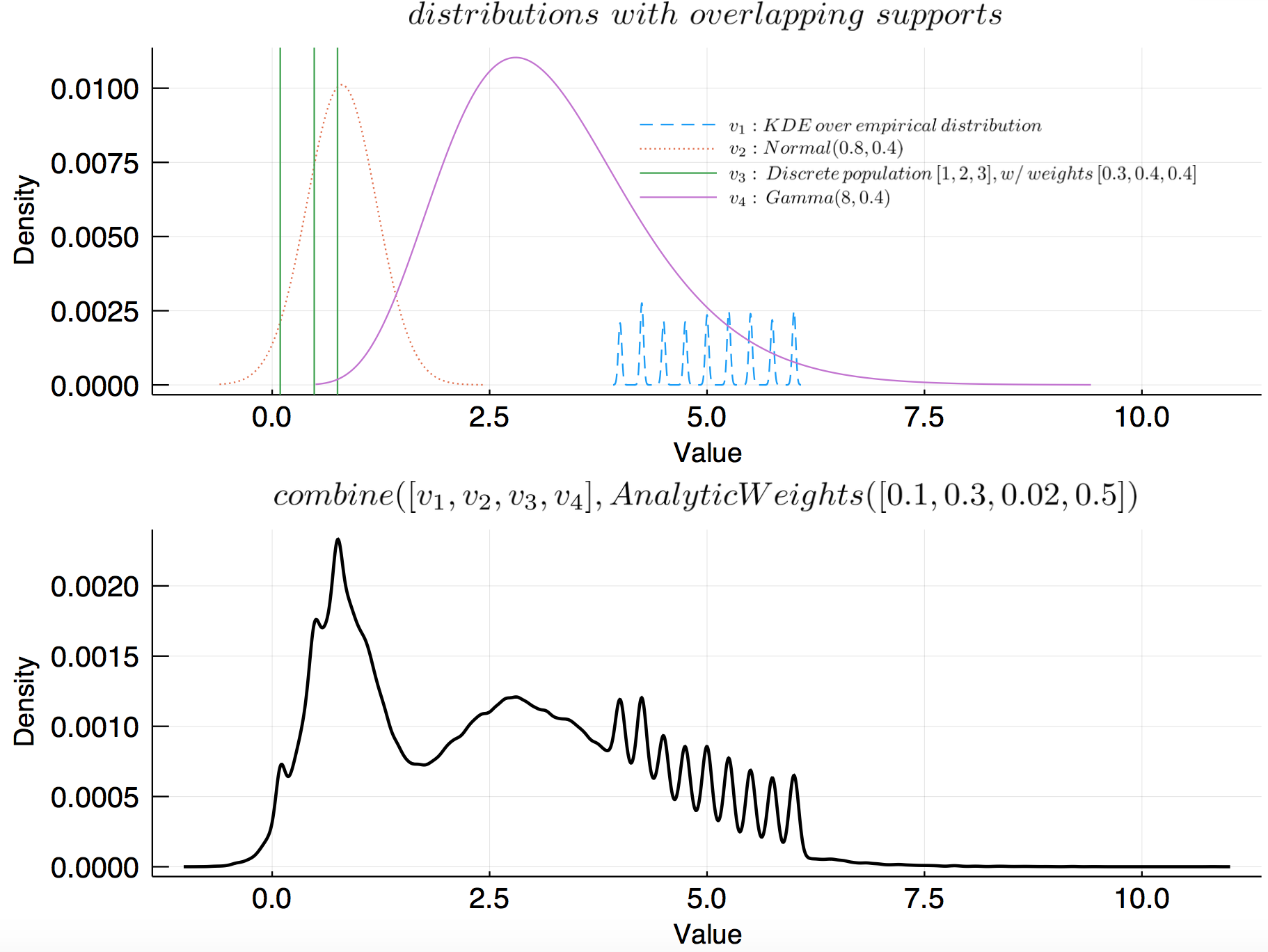
AnalyticWeights
#
UncertainData.combine — Method.
1 2 3 | combine(uvals::Vector{AbstractUncertainValue}, weights::AnalyticWeights; n = 10000*length(uvals), bw::Union{Nothing, Real} = nothing) |
Combine multiple uncertain values into a single uncertain value. This is done by resampling each uncertain value in uvals proportionally to the provided relative probability weights (these are normalised by default, so don't need to sum to 1), then pooling these draws together. Finally, a kernel density estimate to the final distribution is computed over the n total draws.
Providing AnalyticWeights leads to the exact same behaviour as for ProbabilityWeights, but may be more appropriote when relative importance weights are assigned subjectively, and not based on quantitative evidence.
The KDE bandwidth is controlled by bw. By default, bw = nothing; in this case, the bandwidth is determined using the KernelDensity.default_bandwidth function.
Tip
For very wide, close-to-normal distributions, the default bandwidth may work well. If you're combining very peaked distributions or discrete populations, however, you may want to lower the bandwidth significantly.
Example
1 2 3 4 5 6 7 8 9 | v1 = UncertainValue(Normal, 1, 0.3) v2 = UncertainValue(Normal, 0.8, 0.4) v3 = UncertainValue([rand() for i = 1:3], [0.3, 0.3, 0.4]) v4 = UncertainValue(Normal, 3.7, 0.8) uvals = [v1, v2, v3, v4]; # Two difference syntax options combine(uvals, AnalyticWeights([0.2, 0.1, 0.3, 0.2])) combine(uvals, aweights([0.2, 0.1, 0.3, 0.2]), n = 20000) # adjust number of total draws |
For example:
1 2 3 4 5 6 7 8 9 10 11 12 13 14 15 16 17 18 19 20 | v1 = UncertainValue(UnivariateKDE, rand(4:0.25:6, 1000), bandwidth = 0.02) v2 = UncertainValue(Normal, 0.8, 0.4) v3 = UncertainValue([rand() for i = 1:3], [0.3, 0.3, 0.4]) v4 = UncertainValue(Gamma, 8, 0.4) uvals = [v1, v2, v3, v4]; p = plot(title = L"distributions \,\, with \,\, overlapping \,\, supports") plot!(v1, label = L"v_1: KDE \, over \, empirical \, distribution", ls = :dash) plot!(v2, label = L"v_2: Normal(0.8, 0.4)", ls = :dot) vline!(v3.values, label = L"v_3: \, Discrete \, population\, [1,2,3], w/ \, weights \, [0.3, 0.4, 0.4]") # plot each possible state as vline plot!(v4, label = L"v_4: \, Gamma(8, 0.4)") pcombined = plot(combine(uvals, AnalyticWeights([0.1, 0.3, 0.02, 0.5]), n = 100000, bw = 0.05), title = L"combine([v_1, v_2, v_3, v_4], AnalyticWeights([0.1, 0.3, 0.02, 0.5])", lc = :black, lw = 2) plot(p, pcombined, layout = (2, 1), size = (800, 600), link = :x, ylabel = "Density", tickfont = font(12), legendfont = font(8), fg_legend = :transparent, bg_legend = :transparent) |
Generic Weights
#
UncertainData.combine — Method.
1 2 3 | combine(uvals::Vector{AbstractUncertainValue}, weights::Weights; n = 10000*length(uvals), bw::Union{Nothing, Real} = nothing) |
Combine multiple uncertain values into a single uncertain value. This is done by resampling each uncertain value in uvals proportionally to the provided weights (these are normalised by default, so don't need to sum to 1), then pooling these draws together. Finally, a kernel density estimate to the final distribution is computed over the n total draws.
Providing Weights leads to the exact same behaviour as for ProbabilityWeights and AnalyticalWeights.
The KDE bandwidth is controlled by bw. By default, bw = nothing; in this case, the bandwidth is determined using the KernelDensity.default_bandwidth function.
Tip
For very wide, close-to-normal distributions, the default bandwidth may work well. If you're combining very peaked distributions or discrete populations, however, you may want to lower the bandwidth significantly.
Example
1 2 3 4 5 6 7 8 9 | v1 = UncertainValue(Normal, 1, 0.3) v2 = UncertainValue(Normal, 0.8, 0.4) v3 = UncertainValue([rand() for i = 1:3], [0.3, 0.3, 0.4]) v4 = UncertainValue(Normal, 3.7, 0.8) uvals = [v1, v2, v3, v4]; # Two difference syntax options combine(uvals, Weights([0.2, 0.1, 0.3, 0.2])) combine(uvals, weights([0.2, 0.1, 0.3, 0.2]), n = 20000) # adjust number of total draws |
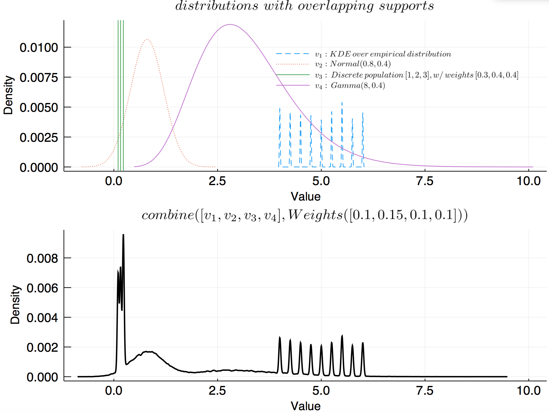
For example:
1 2 3 4 5 6 7 8 9 10 11 12 13 14 15 16 17 18 19 20 21 22 23 | v1 = UncertainValue(UnivariateKDE, rand(4:0.25:6, 1000), bandwidth = 0.01) v2 = UncertainValue(Normal, 0.8, 0.4) v3 = UncertainValue([rand() for i = 1:3], [0.3, 0.3, 0.4]) v4 = UncertainValue(Gamma, 8, 0.4) uvals = [v1, v2, v3, v4]; p = plot(title = L"distributions \,\, with \,\, overlapping \,\, supports") plot!(v1, label = L"v_1: KDE \, over \, empirical \, distribution", ls = :dash) plot!(v2, label = L"v_2: Normal(0.8, 0.4)", ls = :dot) # plot each possible state as vline vline!(v3.values, label = L"v_3: \, Discrete \, population\, [1,2,3], w/ \, weights \, [0.3, 0.4, 0.4]") plot!(v4, label = L"v_4: \, Gamma(8, 0.4)") pcombined = plot(combine(uvals, Weights([0.1, 0.15, 0.1, 0.1]), n = 100000, bw = 0.02), title = L"combine([v_1, v_2, v_3, v_4], Weights([0.1, 0.15, 0.1, 0.1]))", lc = :black, lw = 2) plot(p, pcombined, layout = (2, 1), size = (800, 600), link = :x, ylabel = "Density", tickfont = font(12), legendfont = font(8), fg_legend = :transparent, bg_legend = :transparent) |
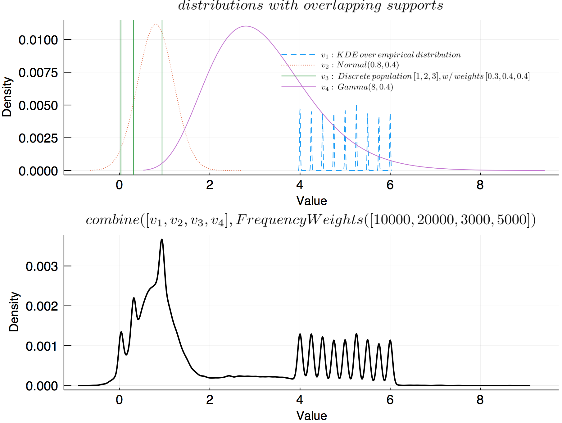
FrequencyWeights
Using FrequencyWeights, one may specify the number of times each of the uncertain values should be sampled to form the pooled resampled draws on which the final kernel density estimate is performed.
#
UncertainData.combine — Method.
1 2 | combine(uvals::Vector{AbstractUncertainValue}, weights::FrequencyWeights; bw::Union{Nothing, Real} = nothing) |
Combine multiple uncertain values into a single uncertain value. This is done by resampling each uncertain value in uvals according to their relative frequencies (the absolute number of draws provided by weights). Finally, a kernel density estimate to the final distribution is computed over the sum(weights) total draws.
The KDE bandwidth is controlled by bw. By default, bw = nothing; in this case, the bandwidth is determined using the KernelDensity.default_bandwidth function.
Tip
For very wide and close-to-normal distributions, the default bandwidth may work well. If you're combining very peaked distributions or discrete populations, however, you may want to lower the bandwidth significantly.
Example
1 2 3 4 5 6 7 8 9 | v1 = UncertainValue(Normal, 1, 0.3) v2 = UncertainValue(Normal, 0.8, 0.4) v3 = UncertainValue([rand() for i = 1:3], [0.3, 0.3, 0.4]) v4 = UncertainValue(Normal, 3.7, 0.8) uvals = [v1, v2, v3, v4]; # Two difference syntax options combine(uvals, FrequencyWeights([100, 500, 343, 7000])) combine(uvals, pweights([1410, 550, 223, 801])) |
For example:
1 2 3 4 5 6 7 8 9 10 11 12 13 14 15 16 17 18 19 20 21 22 23 | v1 = UncertainValue(UnivariateKDE, rand(4:0.25:6, 1000), bandwidth = 0.01) v2 = UncertainValue(Normal, 0.8, 0.4) v3 = UncertainValue([rand() for i = 1:3], [0.3, 0.3, 0.4]) v4 = UncertainValue(Gamma, 8, 0.4) uvals = [v1, v2, v3, v4]; p = plot(title = L"distributions \,\, with \,\, overlapping \,\, supports") plot!(v1, label = L"v_1: KDE \, over \, empirical \, distribution", ls = :dash) plot!(v2, label = L"v_2: Normal(0.8, 0.4)", ls = :dot) # plot each possible state as vline vline!(v3.values, label = L"v_3: \, Discrete \, population\, [1,2,3], w/ \, weights \, [0.3, 0.4, 0.4]") plot!(v4, label = L"v_4: \, Gamma(8, 0.4)") pcombined = plot(combine(uvals, FrequencyWeights([10000, 20000, 3000, 5000]), bw = 0.05), title = L"combine([v_1, v_2, v_3, v_4], FrequencyWeights([10000, 20000, 3000, 5000])", lc = :black, lw = 2) plot(p, pcombined, layout = (2, 1), size = (800, 600), link = :x, ylabel = "Density", tickfont = font(12), legendfont = font(8), fg_legend = :transparent, bg_legend = :transparent) |